Oceanic Basin Modes: Quasi-Geostrophic approach
This tutorial was contributed by Christine Kaufhold and Francis Poulin. The tutorial was later updated by Emma Rothwell to add in the restrict flag in the LinearEigenproblem.
As a continuation of the Quasi-Geostrophic (QG) model described in the other tutorial, we will now see how we can use Firedrake to compute the spatial structure and frequencies of the freely evolving modes in this system, what are referred to as basin modes. Oceanic basin modes are low frequency structures that propagate zonally in the oceans that alter the dynamics of Western Boundary Currents, such as the Gulf Stream. In this particular tutorial we will show how to solve the QG eigenvalue problem with no basic state and no dissipative forces. Unlike the other demo that integrated the equations forward in time, in this problem it is necessary to compute the eigenvalues and eigenfunctions for a particular differential operator.
This demo requires SLEPc and slepc4py to be installed. For instructions on how to install them please follow these instructions.
Governing PDE
We first briefly recap the nonlinear, one-layer QG equation that we considered previously. The interested reader can find the derivations in [QGeval-Ped92] and [QGeval-Val06]. This model consists of an evolution equation for the Potential Vorticity, \(q\), and an elliptic problem through which we can determine the streamfunction,
Where \(\psi\) is the stream-function, \(\vec{u}=(u, v)\) is the velocity field, \(q\) is the Potential Vorticity (PV), \(\beta\) is the Coriolis parameter and \(F\) is the rotational Froude number. The velocity field is easily obtained using
We assume that the amplitude of the wave motion is very small, which allows us to linearize the equations of motion and therefore neglect the nonlinear advection,
We look for wave-like solutions that are periodic in time, with a frequency of \(\omega\)
This has the advantage of removing the time derivative from the equation and replacing it with an eigenvalue, \(i \omega\). By substituting the above solution into the QG equation, we can find a complex eigenvalue problem of the form
Weak Formulation
To use a finite element method it is necessary to formulate the weak form and then we can use SLEPc in Firedrake to compute eigenvalue problems easily. To begin, we multiply this equation by a Test Function \(\phi\) and integrate over the domain \(A\).
To remove the Laplacian operator we use integration by parts and the Divergence theorem to obtain
No-normal flow boundary conditions are required and mathematically this means that the streamfunction must be a constant on the boundary. Since the test functions inherit these boundary conditions, \(\hat{\phi} = 0\) on the boundary, the boundary integral vanishes and the weak form becomes,
Firedrake code
Using this form, we can now implement this eigenvalue problem in Firedrake. We start by importing Firedrake.
from firedrake import *
from firedrake.pyplot import tripcolor
We specify the geometry to be a square geometry with \(50\) cells with length \(1\).
Lx   = 1.
Ly   = 1.
n0   = 50
mesh = RectangleMesh(n0, n0, Lx, Ly, reorder=None)
Next we define the function spaces within which our solution will reside.
Vcg = FunctionSpace(mesh,'CG',3)
We impose zero Dirichlet boundary conditions, in a strong sense, which guarantee that we have no-normal flow at the boundary walls.
bc = DirichletBC(Vcg, 0.0, "on_boundary")
The two non-dimensional parameters are the \(\beta\) parameter, set by the sphericity of the Earth, and the Froude number, the relative importance of rotation to stratification.
beta = Constant('1.0')
F    = Constant('1.0')
We define the Test Function \(\phi\) and the Trial Function \(\psi\) in our function space.
phi, psi = TestFunction(Vcg), TrialFunction(Vcg)
To build the weak formulation of our equation we need to build two PETSc
matrices in the form of a generalized eigenvalue problem,
\(A\psi = \lambda M\psi\). This eigenproblem takes restrict=True to help
users to avoid convergence failures by removing eigenvalues on the
boundary, while preserving the original function space for the eigenmodes.
eigenproblem = LinearEigenproblem(
        A=beta*phi*psi.dx(0)*dx,
        M=-inner(grad(psi), grad(phi))*dx - F*psi*phi*dx,
        bcs=bc, restrict=True)
Next we program our eigenvalue solver through the PETSc options system. The first is specifying that we have an generalized eigenvalue problem that is nonhermitian. Then, we ask for the eigenvalues with the largest imaginary part. Finally we set the spectral transform to shift with no target:
opts = {"eps_gen_non_hermitian": None,
        "eps_largest_imaginary": None,
        "st_type": "shift",
        "eps_target": None,
        "st_pc_factor_shift_type": "NONZERO"}
Finally, we build our eigenvalue solver, specifying in this case that we just want to see the first eigenvalue, eigenvector pair:
eigensolver = LinearEigensolver(eigenproblem, n_evals=1,
                                solver_parameters=opts)
Now solve the system. This returns the number of converged eigenvalues.
nconv = eigensolver.solve()
We now get the real and imaginary parts of the eigenvalue and eigenvector for the leading eigenpair (that with the largest in magnitude imaginary part).
lam = eigensolver.eigenvalue(0)
and we gather the corresponding eigenfunctions
eigenmode_real, eigenmode_imag = eigensolver.eigenfunction(0)
We can now list and show plots for the eigenvalues and eigenfunctions that were found.
print("Leading eigenvalue is:", lam)

try:
    import matplotlib.pyplot as plt
    fig, axes = plt.subplots()
    colors = tripcolor(eigenmode_real, axes=axes)
    fig.colorbar(colors)

    fig, axes = plt.subplots()
    colors = tripcolor(eigenmode_imag, axes=axes)
    fig.colorbar(colors)
    plt.show()
except ImportError:
    warning("Matplotlib not available, not plotting eigemodes")
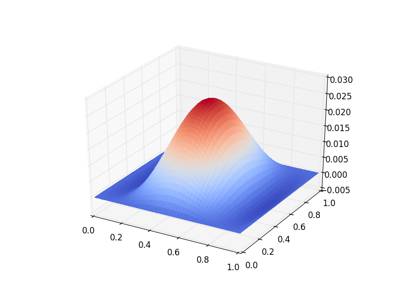
Below is a plot of the spatial structure of the real part of one of the eigenmodes computed above.
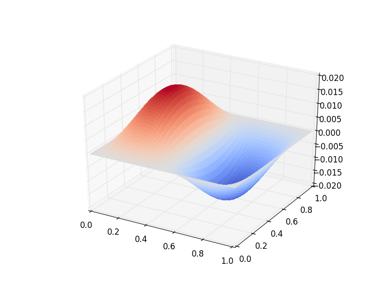
Below is a plot of the spatial structure of the imaginary part of one of the eigenmodes computed above.
This demo can be found as a Python script in qgbasinmodes.py.
References
Joseph Pedlosky. Geophysical Fluid Dynamics. Springer study edition. Springer New York, 1992. ISBN 9780387963877.
Geoffrey K. Vallis. Atmospheric and Oceanic Fluid Dynamics. Cambridge University Press, Cambridge, U.K., 2006.