
Full-waveform inversion: spatial and wave sources parallelism
This tutorial demonstrates a Full-Waveform Inversion (FWI) solver in Firedrake, computing the gradient via algorithmic differentiation. Additionally, we illustrate how to configure spatial and wave source parallelism to efficiently compute the cost functions and their gradients for this optimisation problem.
This tutorial was prepared by Daiane I. Dolci and Jack Betteridge.
FWI consists of a local optimisation, where the goal is to minimise the misfit between observed and predicted seismogram data. The misfit is quantified by a functional, which in general is a summation of the cost functions for multiple wave sources:
where \(N_s\) is the number of sources, and \(J_s(u, u^{obs})\) is the cost function for a single source. Following [Tar84], the cost function for a single source can be measured by:
where \(u = u(c, \mathbf{x}_r,t)\) and \(u_{obs} = u_{obs}(c,\mathbf{x}_r,t)\), are respectively the computed and observed data, both recorded at a finite number of receivers \(N_r\) located at the point positions \(\mathbf{x}_r \in \Omega\), in a time-step interval \([0, T]\), where \(T\) is the total time-step.
The computed data, \(u = u(c, \mathbf{x}_r,t)\), is given on simulating a source wave propagating through an inhomogeneous medium. Here, the wave propagation from a source is modelled by an acoustic wave equation:
where \(m = 1/c^2\), \(c = c(\mathbf{x})\) is the pressure wave velocity, which is assumed here a piecewise-constant and positive. The function \(f_s(\mathbf{x},t)\) models a point source function, were the time-dependency is given by the Ricker wavelet [Ric53].
The acoustic wave equation should satisfy the initial conditions \(u(\mathbf{x}, 0) = 0 = u_t(\mathbf{x}, 0) = 0\). We employ a no-reflective absorbing boundary condition [CE77]:
To solve the wave equation, we consider the following weak form:
for an arbitrary test function \(v\in V\), where \(V\) is a function space.
As shown in (1), the functional \(J\) is a summation of \(J_s\). These functionals \(J_s\) are independent of each other. In Firedrake, it is possible to compute \(J_s\) in parallel. To achieve this, we use ensemble parallelism, which involves solving simultaneous copies of the wave equation (3) with different forcing terms \(f_s(\mathbf{x}, t)\), different \(J_s\) and their gradients (which we will discuss later).
Instantiating an ensemble requires a communicator (usually MPI_COMM_WORLD) plus the number of MPI processes to be used in each member of the ensemble (2, in this case):
from firedrake import *
M = 2
my_ensemble = Ensemble(COMM_WORLD, M)
Each ensemble member will have the same spatial parallelism with the number of ensemble members given
by dividing the size of the original communicator by the number processes in each ensemble member.
In this example, we want to distribute each mesh over 2 ranks and compute the functional and its gradient
for 3 wave sources. Therefore, we will have 3 emsemble members, each with 2 ranks. The total number of
processes launched by mpiexec must therefore be equal to the product of number of ensemble members
(3, in this case) with the number of processes to be used for each ensemble member (M=2, in this case).
Additional details about the ensemble parallelism can be found in the
Firedrake documentation.
The subcommunicators in each ensemble member are: Ensemble.comm and Ensemble.ensemble_comm.
Ensemble.comm is the spatial communicator. Ensemble.ensemble_comm allows communication between
the ensemble members. In this example, Ensemble.ensemble_comm benefits the communication of the
functionals \(J_s\) and their gradients for the distinct the wave sources.
The number of sources is defined with my_ensemble.ensemble_comm.size (3 in this case):
num_sources = my_ensemble.ensemble_comm.size
The source number is defined with the Ensemble.ensemble_comm rank:
source_number = my_ensemble.ensemble_comm.rank
In this example, we consider a two-dimensional square domain with a side length of 1.0 km. The mesh is
built over the my_ensemble.comm (spatial) communicator.
import os
if os.getenv("FIREDRAKE_CI") == "1":
    # Setup for a faster test execution.
    dt = 0.03  # time step in seconds
    final_time = 0.6  # final time in seconds
    nx, ny = 15, 15
else:
    dt = 0.002  # time step in seconds
    final_time = 1.0  # final time in seconds
    nx, ny = 80, 80

mesh = UnitSquareMesh(nx, ny, comm=my_ensemble.comm)
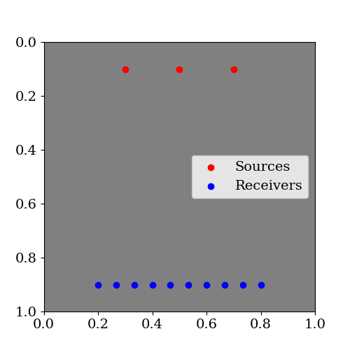
The frequency of the Ricker wavelet, the source and receiver locations are defined as follows:
import numpy as np
frequency_peak = 7.0  # The dominant frequency of the Ricker wavelet in Hz.
source_locations = np.linspace((0.3, 0.1), (0.7, 0.1), num_sources)
receiver_locations = np.linspace((0.2, 0.9), (0.8, 0.9), 20)
Sources and receivers locations are illustrated in the following figure:
FWI seeks to estimate the pressure wave velocity based on the observed data stored at the receivers.
These data are subject to influences of the subsurface medium while waves propagate from the sources.
In this example, we emulate observed data by executing the acoustic wave equation with a synthetic
pressure wave velocity model. The synthetic pressure wave velocity model is referred to here as the
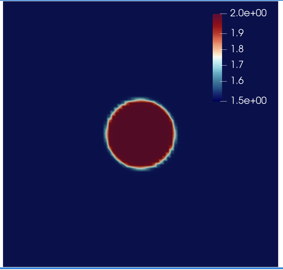
true velocity model (c_true). For the sake of simplicity, we consider c_true consisting of a
circle in the centre of the domain, as shown in the following code cell:
V = FunctionSpace(mesh, "KMV", 1)
x, z = SpatialCoordinate(mesh)
c_true = Function(V).interpolate(1.75 + 0.25 * tanh(200 * (0.125 - sqrt((x - 0.5) ** 2 + (z - 0.5) ** 2))))
To model the point source function in weak form, which is the term on the right side of Eq. (5) rewritten as:
where \(r(t)\) is the Ricker wavelet coded as follows:
def ricker_wavelet(t, fs, amp=1.0):
    ts = 1.5
    t0 = t - ts * np.sqrt(6.0) / (np.pi * fs)
    return (amp * (1.0 - (1.0 / 2.0) * (2.0 * np.pi * fs) * (2.0 * np.pi * fs) * t0 * t0)
            * np.exp((-1.0 / 4.0) * (2.0 * np.pi * fs) * (2.0 * np.pi * fs) * t0 * t0))
To compute the cofunction \(q_s(\mathbf{x})\in V^{\ast}\), we first construct the source mesh over the
source location \(\mathbf{x}_s\), for the source number source_number:
source_mesh = VertexOnlyMesh(mesh, [source_locations[source_number]])
Next, we define a function space \(V_s\) accordingly:
V_s = FunctionSpace(source_mesh, "DG", 0)
The point source value \(d_s(\mathbf{x}_s) = 1.0\) is coded as:
d_s = Function(V_s)
d_s.interpolate(1.0)
We then interpolate a cofunction in \(V_s^{\ast}\) onto \(V^{\ast}\) to then have \(q_s \in V^{\ast}\):
source_cofunction = assemble(d_s * TestFunction(V_s) * dx)
q_s = Cofunction(V.dual()).interpolate(source_cofunction)
The forward wave equation solver is written as follows:
import finat

def wave_equation_solver(c, source_function, dt, V):
    u = TrialFunction(V)
    v = TestFunction(V)
    u_np1 = Function(V) # timestep n+1
    u_n = Function(V) # timestep n
    u_nm1 = Function(V) # timestep n-1
    # Quadrature rule for lumped mass matrix.
    quad_rule = finat.quadrature.make_quadrature(V.finat_element.cell, V.ufl_element().degree(), "KMV")
    m = (1 / (c * c))
    time_term =  m * (u - 2.0 * u_n + u_nm1) / Constant(dt**2) * v * dx(scheme=quad_rule)
    nf = (1 / c) * ((u_n - u_nm1) / dt) * v * ds
    a = dot(grad(u_n), grad(v)) * dx(scheme=quad_rule)
    F = time_term + a + nf
    lin_var = LinearVariationalProblem(lhs(F), rhs(F) + source_function, u_np1)
    # Since the linear system matrix is diagonal, the solver parameters are set to construct a solver,
    # which applies a single step of Jacobi preconditioning.
    solver_parameters = {"mat_type": "matfree", "ksp_type": "preonly", "pc_type": "jacobi"}
    solver = LinearVariationalSolver(lin_var,solver_parameters=solver_parameters)
    return solver, u_np1, u_n, u_nm1
You can find more details about the wave equation with mass lumping on this Firedrake demos.
The receivers mesh and its function space \(V_r\):
receiver_mesh = VertexOnlyMesh(mesh, receiver_locations)
V_r = FunctionSpace(receiver_mesh, "DG", 0)
The receiver mesh is required in order to interpolate the wave equation solution at the receivers.
We are now able to proceed with the synthetic data computations and record them on the receivers:
from firedrake.__future__ import interpolate

true_data_receivers = []
total_steps = int(final_time / dt) + 1
f = Cofunction(V.dual())  # Wave equation forcing term.
solver, u_np1, u_n, u_nm1 = wave_equation_solver(c_true, f, dt, V)
interpolate_receivers = interpolate(u_np1, V_r)

for step in range(total_steps):
    f.assign(ricker_wavelet(step * dt, frequency_peak) * q_s)
    solver.solve()
    u_nm1.assign(u_n)
    u_n.assign(u_np1)
    true_data_receivers.append(assemble(interpolate_receivers))
Next, the FWI problem is executed with the following steps:
Set the initial guess for the parameter
c_guess;Solve the wave equation with the initial guess velocity model (
c_guess);Compute the functional \(J\);
Compute the adjoint-based gradient of \(J\) with respect to the control parameter
c_guess;Update the parameter
c_guessusing a gradient-based optimisation method, on this case the L-BFGS-B method;Repeat steps 2-5 until the optimisation stopping criterion is satisfied.
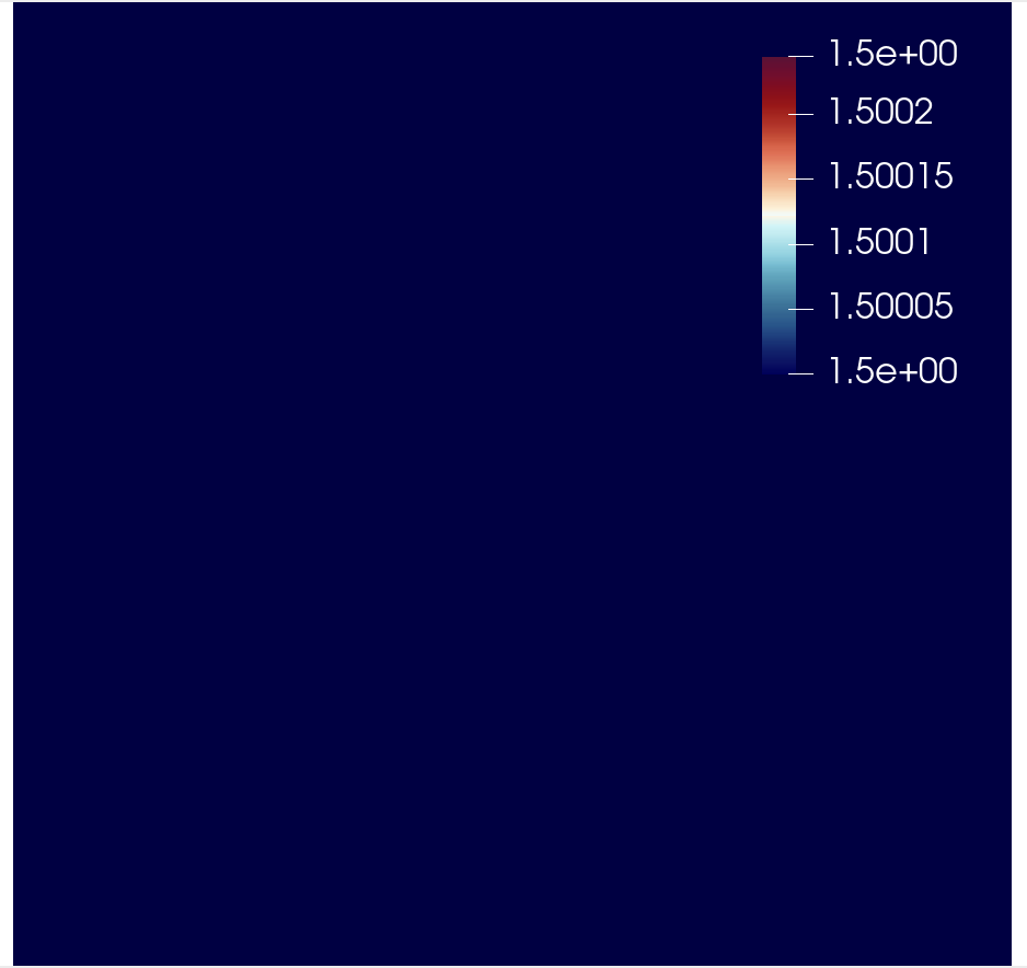
Step 1: The initial guess is set as a constant field with a value of 1.5 km/s:
c_guess = Function(V).interpolate(1.5)
To have the step 4, we need first to tape the forward problem. That is done by calling:
from firedrake.adjoint import *
continue_annotation()
get_working_tape().progress_bar = ProgressBar
Steps 2-3: Solve the wave equation and compute the functional:
f = Cofunction(V.dual())  # Wave equation forcing term.
solver, u_np1, u_n, u_nm1 = wave_equation_solver(c_guess, f, dt, V)
interpolate_receivers = interpolate(u_np1, V_r)
J_val = 0.0
for step in range(total_steps):
    f.assign(ricker_wavelet(step * dt, frequency_peak) * q_s)
    solver.solve()
    u_nm1.assign(u_n)
    u_n.assign(u_np1)
    guess_receiver = assemble(interpolate_receivers)
    misfit = guess_receiver - true_data_receivers[step]
    J_val += 0.5 * assemble(inner(misfit, misfit) * dx)
We now instantiate EnsembleReducedFunctional:
J_hat = EnsembleReducedFunctional(J_val, Control(c_guess), my_ensemble)
which enables us to recompute \(J\) and its gradient \(\nabla_{\mathtt{c\_guess}} J\),
where the \(J_s\) and its gradients \(\nabla_{\mathtt{c\_guess}} J_s\) are computed in parallel
based on the my_ensemble configuration.
Steps 4-6: The instance of the EnsembleReducedFunctional, named J_hat,
is then passed as an argument to the minimize function:
c_optimised = minimize(J_hat, method="L-BFGS-B", options={"disp": True, "maxiter": 1},
                        bounds=(1.5, 2.0), derivative_options={"riesz_representation": 'l2'}
                        )
The minimize function executes the optimisation algorithm until the stopping criterion (maxiter) is met.
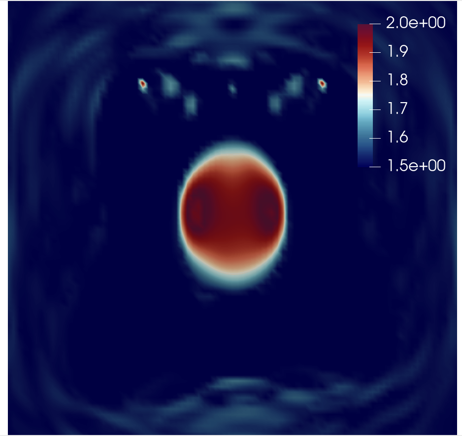
For 20 iterations, the predicted velocity model is shown in the following figure.
Warning
The minimize function uses the SciPy library for optimisation. However, for scenarios that require higher
levels of spatial parallelism, you should assess whether SciPy is the most suitable option for your problem.
SciPy’s optimisation algorithm is not inner-product-aware. Therefore, we configure the options with
derivative_options={"riesz_representation": 'l2'} to account for this requirement.
Note
This example is only a starting point to help you to tackle more intricate FWI problems.
References
Robert Clayton and Björn Engquist. Absorbing boundary conditions for acoustic and elastic wave equations. Bulletin of the seismological society of America, 67(6):1529–1540, 1977. doi:https://doi.org/10.1785/BSSA0670061529.
Norman Ricker. The form and laws of propagation of seismic wavelets. Geophysics, 18(1):10–40, 1953. doi:https://doi.org/10.1190/1.1437843.
Albert Tarantola. Inversion of seismic reflection data in the acoustic approximation. Geophysics, 49(8):1259–1266, 1984. doi:https://doi.org/10.1190/1.1441754.