The \(R\) space

The function space \(R\) (for “Real”) is the space of functions which are constant over the whole domain. It is employed to model concepts such as global constraints.

An example:

Warning

This section illustrates the use of the Real space using the simplest example. This is usually not the optimal approach for removing the nullspace of an operator. If that is your only goal then you are probably better placed removing the null space in the linear solver using the facilities documented in the section Solving singular systems.

Consider a Poisson equation in weak form, find \(u\in V\) such that:

\[\int_\Omega \nabla u \cdot \nabla v \,\mathrm{d}x = -\int_{\Gamma(3)} v\,\mathrm{d}s + \int_{\Gamma(4)} v\,\mathrm{d}s \qquad\forall v\in V\]

where \(\Gamma(3)\) and \(\Gamma(4)\) are domain boundaries over which the boundary conditions \(\nabla u \cdot n = -1\) and \(\nabla u \cdot n = 1\) are applied respectively. This system has a null space composed of the constant functions. One way to remove this is to add a Lagrange multiplier from the space \(R\) and use the resulting constraint equation to enforce that the integral of \(u\) is zero. The resulting system is find \(u\in V\), \(r\in R\) such that:

\[ \begin{align}\begin{aligned}\int_\Omega \nabla u \cdot \nabla v + rv\,\mathrm{d}x = -\int_{\Gamma(3)} v\,\mathrm{d}s + \int_{\Gamma(4)} v\,\mathrm{d}s \qquad\forall v\in V\\\int_\Omega us \,\mathrm{d}x = 0 \qquad \forall s\in R\end{aligned}\end{align} \]

The corresponding Python code is:

from firedrake import *

m = UnitSquareMesh(25, 25)
V = FunctionSpace(m, 'CG', 1)
R = FunctionSpace(m, 'R', 0)
W = V * R
u, r = TrialFunctions(W)
v, s = TestFunctions(W)

a = inner(grad(u), grad(v))*dx + u*s*dx + v*r*dx
L = -v*ds(3) + v*ds(4)

w = Function(W)
solve(a == L, w)
u, s = split(w)
exact = Function(V)
x, y = SpatialCoordinate(m)
exact.interpolate(y - 0.5)
print(sqrt(assemble((u - exact)*(u - exact)*dx)))

Setting and retrieving the value of a function in \(R\)

Functions in the space \(R\) are equivalent to a single floating point value. The value can be set using the Assigner.assign() method of Firedrake functions, and the value can be accessed simply by casting it to float:

from firedrake import *

m = UnitSquareMesh(25, 25)
R = FunctionSpace(m, 'R', 0)

f = Function(V)
f.assign(2.0)
print(float(f))

Note

The \(R\) space is not currently supported in complex mode.

Representing matrices involving \(R\)

Functions in the space \(R\) are different from other finite element functions in that their support extends to the whole domain. To illustrate the consequences of this, we can represent the matrix in the Poisson problem above as:

\[\begin{split}A= \begin{bmatrix} L & K \\ K^T & 0 \end{bmatrix}\end{split}\]

where:

\[ \begin{align}\begin{aligned}L_{ij} = \int_\Omega \nabla \phi_i \phi_j \,\mathrm{d}x\\K_{ij} = \int_\Omega \phi_i \psi_j \,\mathrm{d}x\end{aligned}\end{align} \]

where \(\{\phi_i\}\) is the basis for \(V\) and \(\{\psi_i\}\) is the basis for \(R\). Note that there is only a single basis function for \(R\) and \(\psi_i \equiv 1\) hence:

\[K_{ij} = \int_\Omega \phi_i \,\mathrm{d}x\]

with the result that \(K\) is a single dense matrix column. Similiarly, \(K^T\) is a single dense matrix row.

Using the CSR matrix format typically employed by Firedrake, each matrix row is stored on a single processor. Were this carried through to \(K^T\), both the assembly and action of this row would require the entire system state to be gathered onto one MPI process. This is clearly a horribly non-performant option.

Instead, we observe that a dense matrix row (or column) is isomorphic to a Function and implement these matrix blocks accordingly.

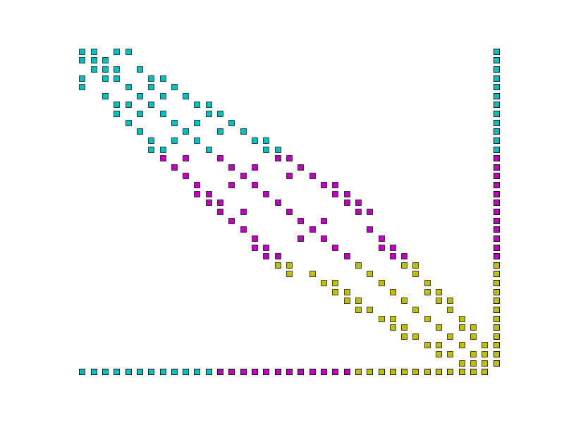
Example parallel distribution of the matrix \(A\). Colours indicate the processor on which the data is stored. Notice the dense row and column, and that the dense row is distributed across the processors.

Assembling matrices involving \(R\)

Assembling the column block is implemented by replacing the trial function with the constant 1, thereby transforming a 2-form into a 1-form, and assembling. Similarly, assembling the row block simply requires the replacement of the test function with the constant 1, and assembling.

The one by one block in the corner is assembled by replacing both the test and trial functions of the corresponding form with 1 and assembling. The remaining block does not involve \(R\) and is assembled as usual.

Using \(R\) space with extruded meshes

On extruded meshes it is possible to construct tensor product function spaces with the \(R\) space. Using the \(R\) space in the extruded direction provides a convenient way of expressing fields that are constant along the extrusion.

The example below illustrates how the \(R\) space can be used to compute a vertical average of a three-dimensional DG1 field by projecting the source field on a DG1 x R space.

from firedrake import *

mesh2d = UnitSquareMesh(10, 10)
mesh = ExtrudedMesh(mesh2d, 10, 0.1)

V = FunctionSpace(mesh, 'DG', 1, vfamily='DG', vdegree=1)
f = Function(V)
x, y, z = SpatialCoordinate(mesh)
f.interpolate(sin(2*pi*z))

U = FunctionSpace(mesh, 'DG', 1, vfamily='R', vdegree=0)
g = Function(U, name='g')
g.project(f)

print('f min: {:.3g}, max: {:.3g} '.format(f.dat.data.min(), f.dat.data.max()))
print('g min: {:.3g}, max: {:.3g} '.format(g.dat.data.min(), g.dat.data.max()))