
Extruded Meshes in Firedrake
Introduction
Firedrake provides several utility functions for the creation of semi-structured meshes from an unstructured base mesh. Firedrake also provides a wide range of finite element spaces, both simple and sophisticated, for use with such meshes.
These meshes may be particularly appropriate when carrying out simulations on high aspect ratio domains. More mundanely, they allow a two-dimensional mesh to be built from square or rectangular cells.
The partial structure can be exploited to give performance advantages when iterating over the mesh, relative to a fully unstructured traversal of the same mesh. Firedrake exploits these benefits when extruded meshes are used.
Structured, Unstructured and Semi-Structured Meshes
Structured and unstructured meshes differ in the way the topology of the mesh is specified.
In a fully structured mesh, the array indices of mesh entities can be computed directly. For example, given the index of the current cell, the indices of the cell’s vertices can be computed using a simple mathematical expression. This means that data can be directly addressed, using expressions of the form A[i].
In a fully unstructured mesh, there is no simple relation between the indices of different mesh entities. Instead, the relationships have to be explicitly stored. For example, given the index of the current cell, the indices of the cell’s vertices can only be found by looking up the information in a separate array. It follows that data must be indirectly addressed, using expressions of the form A[B[i]].
Memory access latency makes indirect addressing more expensive than direct addressing: it is usually more efficient to compute the array index directly than to look it up from memory.
The characteristics of a semi-structured or extruded mesh lie somewhere between the two extremes above. An extruded mesh has an unstructured base mesh. Each cell of the base mesh corresponds to a column of cells in the extruded mesh. Visiting the first cell in each column requires indirect addressing. However, visiting subsequent cells in the column can be done using direct addressing. As the number of cells in the column increases, the performance should approach that of a fully structured mesh.
Generating Extruded Meshes in Firedrake
Extruded meshes are built using ExtrudedMesh(). There
are several built-in extrusion types that generate commonly-used extruded
meshes. To create a more complicated extruded mesh, one can either pass a
hand-written kernel to ExtrudedMesh(), or one
can use a built-in extrusion type and modify the coordinate field afterwards.
The following information may be passed in to the constructor:
a
Meshobject, which will be used as the base mesh.the desired number of cell layers in the extruded mesh. One may also specify layers per column, see below for more information.
the
extrusion_type, which can be one of the built-in “uniform”, “radial” or “radial_hedgehog” – these are described below – or “custom”. If this argument is omitted, the “uniform” extrusion type will be used.the
layer_height, which is needed for the built-in extrusion types.a
kernel, only if the custom extrusion type is usedthe appropriate
gdim, describing the geometric dimension of the mesh, only if the custom extrusion type is used.
Uniform Extrusion
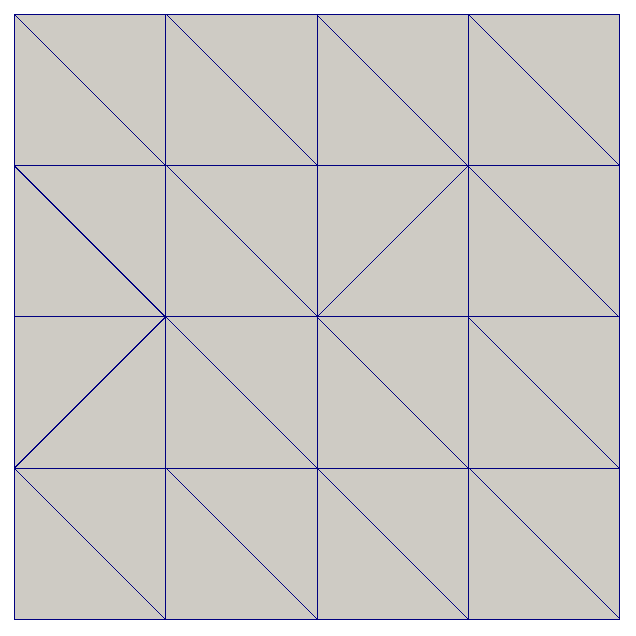
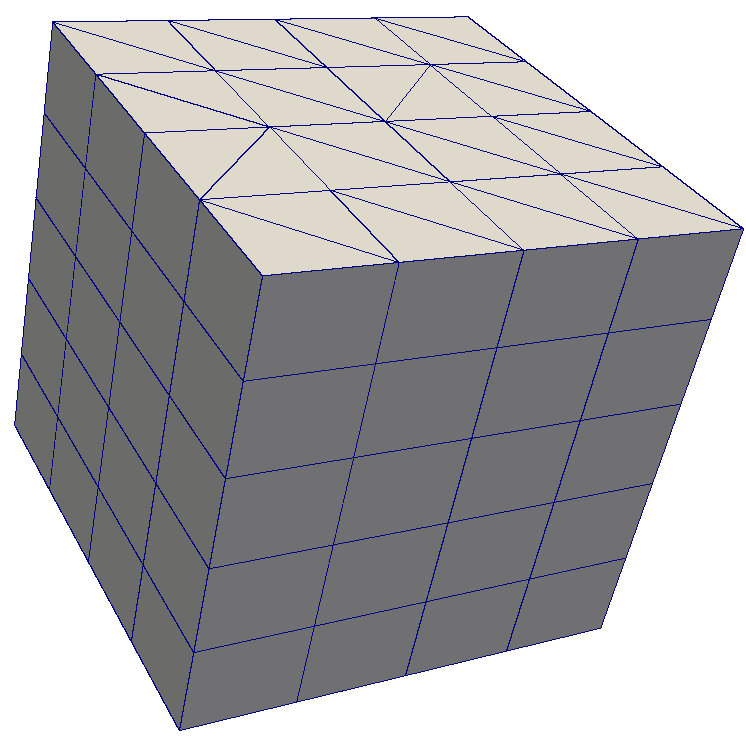
Uniform extrusion adds another spatial dimension to the mesh. For example, a 2D base mesh becomes a 3D extruded mesh. The coordinates of the extruded mesh are computed on the assumption that the layers are evenly spaced (hence the word ‘uniform’).
Let m be a standard UnitSquareMesh(). The following code
produces the extruded mesh, whose base mesh is m, with 5 mesh layers and
a layer thickness of 0.2:
m = UnitSquareMesh(4, 4)
mesh = ExtrudedMesh(m, 5, layer_height=0.2, extrusion_type='uniform')
This can be simplified slightly. The extrusion_type defaults to ‘uniform’, so this can be omitted. Furthermore, the layer_height, if omitted, defaults to the reciprocal of the number of layers. The following code therefore has the same effect:
m = UnitSquareMesh(4, 4)
mesh = ExtrudedMesh(m, 5)
The base mesh and extruded mesh are shown below.
Radial Extrusion
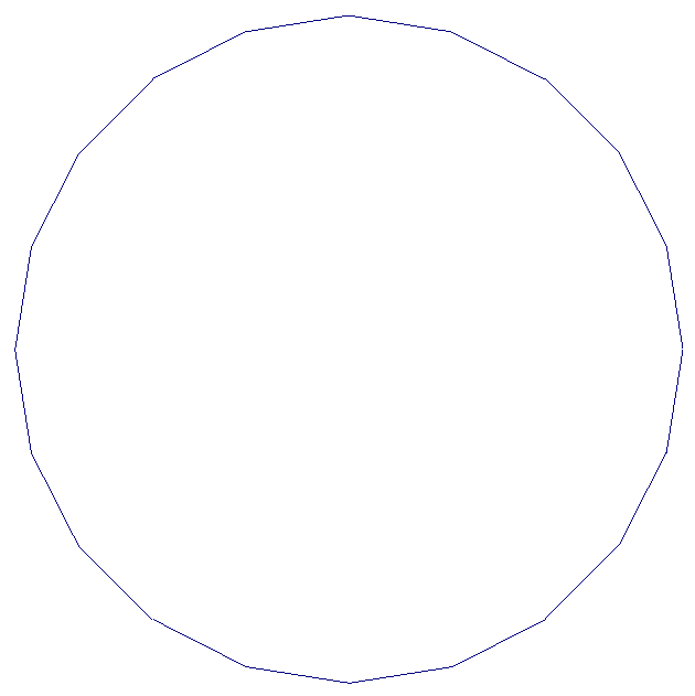
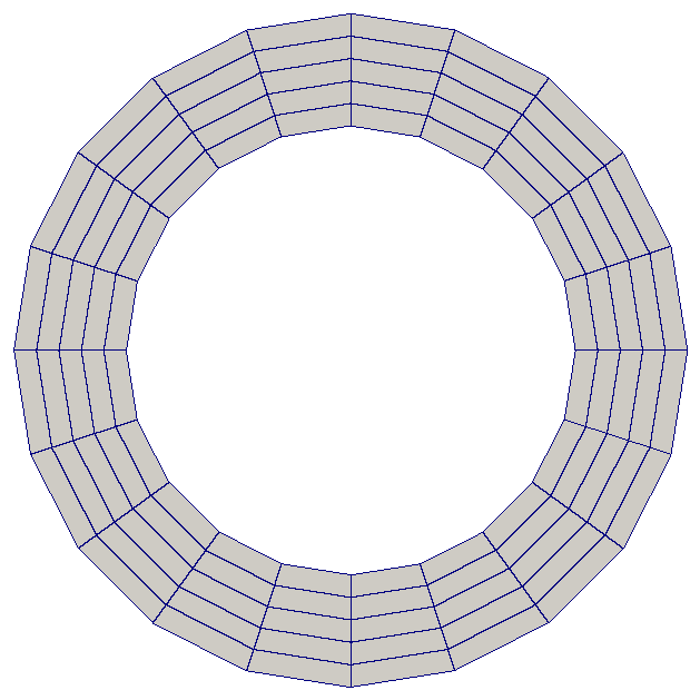
Radial extrusion extrudes cells radially outwards from the origin, without increasing the number of spatial dimensions. An example in 2 dimensions, in which a circle is extruded into an annulus, is:
m = CircleManifoldMesh(20, radius=2)
mesh = ExtrudedMesh(m, 5, extrusion_type='radial')
The base mesh and extruded mesh are shown below.
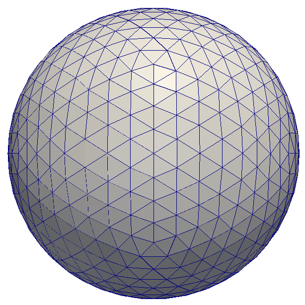
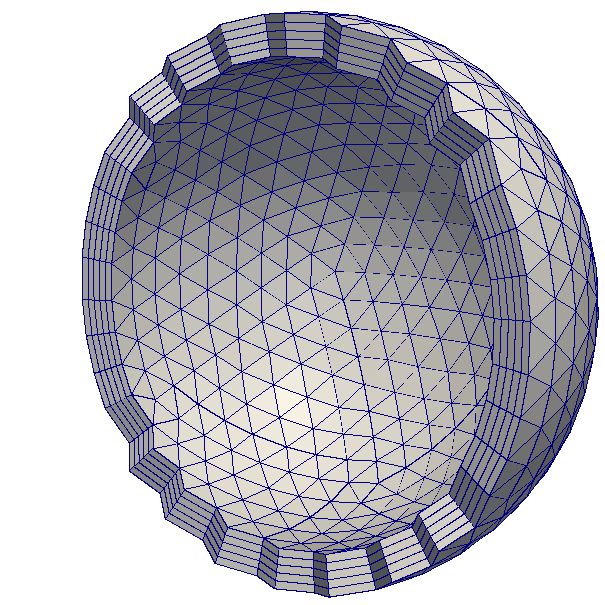
An example in 3 dimensions, in which a sphere is extruded into a spherical annulus, is:
m = IcosahedralSphereMesh(radius=3, refinement_level=3)
mesh = ExtrudedMesh(m, 5, layer_height=0.1, extrusion_type='radial')
The base mesh and part of the extruded mesh are shown below.
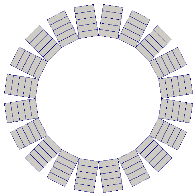
Hedgehog Extrusion
Hedgehog extrusion is similar to radial extrusion, but the cells are extruded outwards in a direction normal to the base cell. This produces a discontinuous coordinate field.
m = CircleManifoldMesh(20, radius=2)
mesh = ExtrudedMesh(m, 5, extrusion_type='radial_hedgehog')
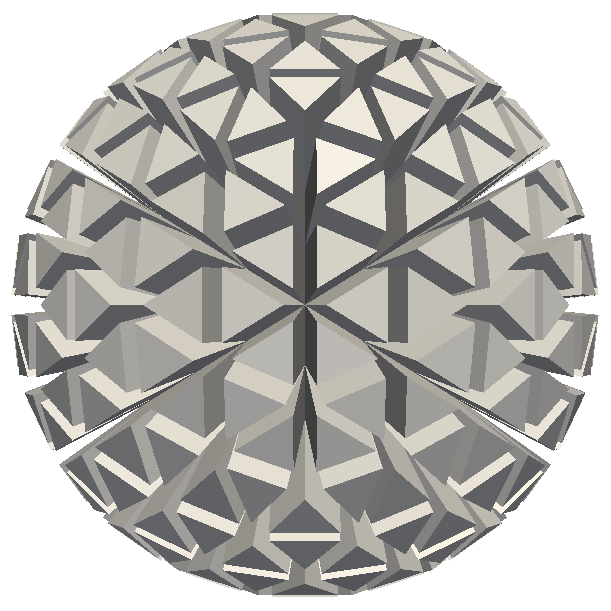
An example in 3 dimensions, in which a sphere is extruded into a spherical annulus, is:
m = UnitIcosahedralSphereMesh(refinement_level=2)
mesh = ExtrudedMesh(m, 5, layer_height=0.1, extrusion_type='radial_hedgehog')
The 2D and 3D hedgehog-extruded meshes are shown below.
Changing coordinates
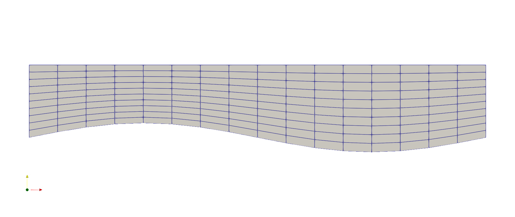
A common use case is that the bottom and/or top of the domain is not flat (or spherical) but is given by a spatially varying field defined on the base mesh. In this case, a straightforward approach is to uniformly extrude to a unit height, and then to create a new coordinate field by changing coordinates to conform to the bathymetry. The example below shows how to do this. This could be combined with interpolation from external data to incorporate domain boundary data from any source. Naturally, the change of coordinates can also be varied to produce a non-uniform distribution of the mesh layers.
base_mesh = IntervalMesh(16, 0, 2*pi)
# Make a height 1 mesh.
unit_extruded_mesh = ExtrudedMesh(base_mesh, layers=10)

base_fs = FunctionSpace(base_mesh, "CG", 1)

x, = SpatialCoordinate(base_mesh)
# You could set this field any way you like.
bathymetry = assemble(interpolate(0.2*sin(x), base_fs))

# Now we transfer the bathymetry field into a depth-averaged field.
extruded_element = FiniteElement("R", "interval", 0)
extruded_space = FunctionSpace(unit_extruded_mesh,
                               TensorProductElement(base_fs.ufl_element(),
                                                    extruded_element))
extruded_bathymetry = Function(extruded_space)
extruded_bathymetry.dat.data_wo[:] = bathymetry.dat.data_ro[:]

# Build a new coordinate field by change of coordinates.
x, y = SpatialCoordinate(unit_extruded_mesh)
new_coordinates = assemble(
    interpolate(
        as_vector([x, extruded_bathymetry + y * (1-extruded_bathymetry)]),
        unit_extruded_mesh.coordinates.function_space()
    )
)
# Finally build the mesh you are actually after.
mesh = Mesh(new_coordinates)
The mesh generated in this example is shown below:
Custom Extrusion
For a more complicated extruded mesh, a custom kernel can be given by the user. Since this is a mesh-wide operation, a PyOP2 parallel loop is constructed by Firedrake.
m = UnitSquareMesh(5, 5)
kernel = op2.Kernel("""
    void extrusion_kernel(double **base_coords, double **ext_coords,
                          double *layer_height, int layer) {
        for (int i=0; i<6; i++) {
            ext_coords[i][0] = base_coords[i / 2][0]; // X
            ext_coords[i][1] = base_coords[i / 2][1]; // Y
            ext_coords[i][2] = 0.1 * (layer + (i % 2)) + 0.5 * base_coords[i / 2][1]; // Z
        }
    }
""", "extrusion_kernel")
mesh = ExtrudedMesh(m, 5, extrusion_type='custom', kernel=kernel, gdim=3)
Variable numbers of mesh cell layers
The simplest method of creating an extruded mesh is to provide a constant number of cell layers for every cell in the base mesh. For some applications, this may not provide sufficient flexibility. Firedrake therefore also allows creation of extruded meshes with a different number of cells in each cell column. To do this, we provide an array with two values for each cell in the mesh. The first entry is the number cells offset from the “bottom” (zero) level, the second is the number of cells in the column.
For example, we might create this extruded mesh:
mesh = UnitIntervalMesh(3)
extmesh = ExtrudedMesh(mesh, layers=[[0, 2], [1, 1], [2, 1]],
                       layer_height=0.25)
which results in the following mesh topology.:
                  x--------x
                  |        |
                  |        |
                  |        |
                  |        |
x--------x--------x--------x
|        |        |
|        |        |
|        |        |
|        |        |
x--------x--------x
|        |
|        |
|        |
|        |
x--------x
To simplify the implementation, we never iterate over the interior facets that only have cells on one side. When you construct the mesh, you should arrange that these facets have zero area, by squashing the coordinates together. In addition, we require that the resulting extruded mesh does not contain topologically disconnected columns: offset cells must, at least, share a vertex with some other cell.
Note
When running in parallel, the base mesh will be distributed before the extruded mesh is created. So you should arrange that the layers array that you provide is specified accordingly (matching the parallel distribution).
For more details on the implementation, see
firedrake.cython.extrusion_numbering.
Function Spaces on Extruded Meshes
The syntax for building a FunctionSpace on an extruded mesh is
an extension of the existing syntax used with normal meshes. On a
non-extruded mesh, the following syntax is used:
mesh = UnitSquareMesh(4, 4)
V = FunctionSpace(mesh, "RT", 1)
To allow maximal flexibility in constructing function spaces, Firedrake supports a more general syntax:
V = FunctionSpace(mesh, element)
where element is a UFL FiniteElement object. This
requires generation and manipulation of FiniteElement objects.
Geometrically, an extruded mesh cell is the product of a base, “horizontal”, cell with a “vertical” interval. The construction of function spaces on extruded meshes makes use of this. Firedrake supports all function spaces whose local element can be expressed as the product of an element defined on the base cell with an element defined on an interval.
We will now introduce the new operators which act on FiniteElement objects.
The TensorProductElement operator
To create an element compatible with an extruded mesh, one should use
the TensorProductElement
operator. For example,
horiz_elt = FiniteElement("CG", triangle, 1)
vert_elt = FiniteElement("CG", interval, 1)
elt = TensorProductElement(horiz_elt, vert_elt)
V = FunctionSpace(mesh, elt)
will give a continuous, scalar-valued function space. The resulting space contains functions which vary linearly in the horizontal direction and linearly in the vertical direction.

The product of a CG1 triangle element with a CG1 interval element
The degree and continuity may differ; for example
horiz_elt = FiniteElement("DG", triangle, 0)
vert_elt = FiniteElement("CG", interval, 2)
elt = TensorProductElement(horiz_elt, vert_elt)
V = FunctionSpace(mesh, elt)
will give a function space which is continuous between cells in a column, but discontinuous between horizontally-neighbouring cells. In addition, the function may vary piecewise-quadratically in the vertical direction, but is piecewise constant horizontally.

The product of a DG0 triangle element with a CG2 interval element
A more complicated element, like a Mini horizontal element with linear
variation in the vertical direction, may be built using the
EnrichedElement functionality
in either of the following ways:
mini_horiz_1 = FiniteElement("CG", triangle, 1)
mini_horiz_2 = FiniteElement("B", triangle, 3)
mini_horiz = mini_horiz_1 + mini_horiz_2  # Enriched element
mini_vert = FiniteElement("CG", interval, 1)
mini_elt = TensorProductElement(mini_horiz, mini_vert)
V = FunctionSpace(mesh, mini_elt)
or
mini_horiz_1 = FiniteElement("CG", triangle, 1)
mini_horiz_2 = FiniteElement("B", triangle, 3)
mini_vert = FiniteElement("CG", interval, 1)
mini_elt_1 = TensorProductElement(mini_horiz_1, mini_vert)
mini_elt_2 = TensorProductElement(mini_horiz_2, mini_vert)
mini_elt = mini_elt_1 + mini_elt_2  # Enriched element
V = FunctionSpace(mesh, mini_elt)

The product of a Mini triangle element with a CG1 interval element
The HDivElement and HCurlElement operators
For moderately complicated vector-valued elements,
TensorProductElement
does not give enough information to unambiguously produce the desired
space. As an example, consider the lowest-order Raviart-Thomas element on a
quadrilateral. The degrees of freedom live on the facets, and consist of
a single evaluation of the component of the vector field normal to each facet.
The following element is closely related to the desired Raviart-Thomas element:
CG_1 = FiniteElement("CG", interval, 1)
DG_0 = FiniteElement("DG", interval, 0)
P1P0 = TensorProductElement(CG_1, DG_0)
P0P1 = TensorProductElement(DG_0, CG_1)
elt = P1P0 + P0P1

The element created above
However, this is only scalar-valued. There are two natural vector-valued
elements that can be generated from this: one of them preserves tangential
continuity between elements, and the other preserves normal continuity
between elements. To obtain the Raviart-Thomas element, we must use the
HDivElement operator:
CG_1 = FiniteElement("CG", interval, 1)
DG_0 = FiniteElement("DG", interval, 0)
P1P0 = TensorProductElement(CG_1, DG_0)
RT_horiz = HDivElement(P1P0)
P0P1 = TensorProductElement(DG_0, CG_1)
RT_vert = HDivElement(P0P1)
elt = RT_horiz + RT_vert

The RT quadrilateral element, requiring the use
of HDivElement
Another reason to use these operators is when expanding a vector into a higher dimensional space. Consider the lowest-order Nedelec element of the 2nd kind on a triangle:
N2_1 = FiniteElement("N2curl", triangle, 1)
This is naturally vector-valued, and has two components. Suppose we form the product of this with a continuous element on an interval:
CG_2 = FiniteElement("CG", interval, 2)
N2CG = TensorProductElement(N2_1, CG_2)
This element still only has two components. To expand this into a
three-dimensional curl-conforming element, we must use the
HCurlElement operator; the syntax is:
Ned_horiz = HCurlElement(N2CG)

This gives the horizontal part of a Nedelec edge element on a triangular prism. The full element can be built as follows:
N2_1 = FiniteElement("N2curl", triangle, 1)
CG_2 = FiniteElement("CG", interval, 2)
N2CG = TensorProductElement(N2_1, CG_2)
Ned_horiz = HCurlElement(N2CG)
P2tr = FiniteElement("CG", triangle, 2)
P1dg = FiniteElement("DG", interval, 1)
P2P1 = TensorProductElement(P2tr, P1dg)
Ned_vert = HCurlElement(P2P1)
Ned_wedge = Ned_horiz + Ned_vert
V = FunctionSpace(mesh, Ned_wedge)
Shortcuts for simple spaces
Simple scalar-valued spaces can be created using a variation on the existing
syntax, if the HDivElement, HCurlElement and enrichment operations
are not required. To create a function space of degree 2 in the horizontal
direction, degree 1 in the vertical direction and possibly discontinuous
between layers, the short syntax is
fspace = FunctionSpace(mesh, "CG", 2, vfamily="DG", vdegree=1)
If the horizontal and vertical parts have the same family and degree,
the vfamily and vdegree arguments may be omitted. If mesh is an
ExtrudedMesh then the following are equivalent:
fspace = FunctionSpace(mesh, "Lagrange", 1)
and
fspace = FunctionSpace(mesh, "Lagrange", 1, vfamily="Lagrange", vdegree=1)
Solving Equations on Extruded Meshes
Once the mesh and function spaces have been declared, extruded meshes behave almost identically to normal meshes. However, there are some small differences, which are listed below.
Surface integrals are no longer denoted by
ds. Since extruded meshes have multiple types of surfaces, the following notation is used:ds_vis used to denote an integral over side facets of the mesh. This can be combined with boundary markers from the base mesh, such asds_v(1).ds_tis used to denote an integral over the top surface of the mesh.ds_bis used to denote an integral over the bottom surface of the mesh.ds_tbis used to denote an integral over both the top and bottom surfaces of the mesh.
Interior facet integrals are no longer denoted by
dS. The horizontal and vertical interior facets may require different numerical treatment. To facilitate this, the following notation is used:dS_his used to denote an integral over horizontal interior facets (between cells that are vertically-adjacent).dS_vis used to denote an integral over vertical interior facets (between cells that are horizontally-adjacent).
When setting strong boundary conditions, the boundary markers from the base mesh can be used to set boundary conditions on the relevant side of the extruded mesh. To set boundary conditions on the top or bottom, the label is replaced by:
top, to set a boundary condition on the top surface.bottom, to set a boundary condition on the bottom surface.
Note that for extruded meshes, the label
on_boundaryonly refers to the side boundaries that take their labels from the base mesh, and not the top or bottom boundaries.