
The Monge-Ampère equation
This tutorial was contributed by Colin Cotter, based on code from Andrew McRae and Lawrence Mitchell.
The Monge-Ampère equation provides the solution to the optimal transportation problem between two measures. Here, we consider the case where the target measure is the usual Lebesgue measure, and the template measure is \(f(x)d^nx\), both defined on the same domain. Then, in two dimensions, the optimal transportation plan is given by
where \(u\) satisfies the the Monge-Ampère equation
where \(I\) is the identity matrix, and \(D^2\) is the Hessian matrix of second derivatives, subject to the boundary conditions \(\frac{\partial u}{\partial n}=0\).
Here we follow the approach of [LP13], namely to use the mixed formulation
where \(\sigma\) is a \(2\times 2\) tensor.
Written in weak form, our problem is to find \((u, \sigma) \in V\times \Sigma = W\) such that
This is called a nonvariational discretisation since the PDE is not in a divergence form. Note that we have dropped the boundary terms that vanish due to the boundary condition. To proceed in the discretisation, we simply choose \(V\) to be a continuous degree-k finite element space, and \(\Sigma\) to be the \(2 \times 2\) tensor continuous finite element space of the same degree. Since we have Neumann boundary conditions, this variational problem has a null space consisting of the constant functions in \(V\).
For Dirichlet boundary conditions, [Awa14] proved that this algorithm converges when \(k>1\). Note that the Jacobian system arising from Newton is only elliptic when \(I + \sigma\) is positive-definite; it is observed that positive-definiteness is preserved by Newton iteration and hence we must be careful to choose an appropriate initial guess. This is one of the reasons why we have set things up with \(I + \sigma\) here instead of \(\sigma\) as is more conventional for these equations, since then \(u=0\) is an appropriate initial guess. This setup also makes the application of the weak boundary conditions easier.
We now proceed to set up the problem in Firedrake using a square mesh of quadrilaterals.
from firedrake import *
n = 100
mesh = UnitSquareMesh(n, n, quadrilateral=True)
We construct the quadratic function space for \(u\),
V = FunctionSpace(mesh, "CG", 2)
and the function space for \(\sigma\).
Sigma = TensorFunctionSpace(mesh, "CG", 2)
We then combine them together in a mixed function space.
W = V*Sigma
Next, we set up the source function, which must integrate to the area
of the domain. Note how in the integration of the Constant
one, we must explicitly specify the domain we wish to integrate over.
x, y = SpatialCoordinate(mesh)
fexpr = exp(-(cos(x)**2 + cos(y)**2))
f = Function(V).interpolate(fexpr)
scaling = assemble(Constant(1)*dx(domain=mesh))/assemble(f*dx)
f *= scaling
assert abs(assemble(f*dx)-assemble(Constant(1)*dx(domain=mesh))) < 1.0e-8
Now we build the UFL expression for the variational form. We will use the nonlinear solve, so the form needs to be a 1-form that depends on a Function, w.
v, tau = TestFunctions(W)
w = Function(W)
u, sigma = split(w)

n = FacetNormal(mesh)

I = Identity(mesh.geometric_dimension)

L = inner(sigma, tau)*dx
L += (inner(div(tau), grad(u))*dx
      - (tau[0, 1]*n[1]*u.dx(0) + tau[1, 0]*n[0]*u.dx(1))*ds)
L -= (det(I + sigma) - f)*v*dx
We must specify the nullspace for the operator. First we define a constant nullspace,
V_basis = VectorSpaceBasis(constant=True)
then we use it to build a nullspace of the mixed function space \(W\).
nullspace = MixedVectorSpaceBasis(W, [V_basis, W.sub(1)])
Then we set up the variational problem.
u_prob = NonlinearVariationalProblem(L, w)
We need to set quite a few solver options, so we’ll put them into a dictionary.
sp_it = {
We’ll only use stationary preconditioners in the Schur complement, so we can get away with GMRES applied to the whole mixed system
#
   "ksp_type": "gmres",
We set up a Schur preconditioner, which is of type “fieldsplit”. We also need to tell the preconditioner that we want to eliminate \(\sigma\), which is field “1”, to get an equation for \(u\), which is field “0”.
#
   "pc_type": "fieldsplit",
   "pc_fieldsplit_type": "schur",
   "pc_fieldsplit_0_fields": "1",
   "pc_fieldsplit_1_fields": "0",
The “selfp” option selects a diagonal approximation of the A00 block.
#
   "pc_fieldsplit_schur_precondition": "selfp",
We just use ILU to approximate the inverse of A00, without a KSP solver,
#
   "fieldsplit_0_pc_type": "ilu",
   "fieldsplit_0_ksp_type": "preonly",
and use GAMG to approximate the inverse of the Schur complement matrix.
#
   "fieldsplit_1_ksp_type": "preonly",
   "fieldsplit_1_pc_type": "gamg",
   "fieldsplit_1_mg_levels_pc_type": "sor",
Finally, we’d like to see some output to check things are working, and to limit the KSP solver to 20 iterations.
#
   "ksp_monitor": None,
   "ksp_max_it": 20,
   "snes_monitor": None
   }
We then put all of these options into the iterative solver,
u_solv = NonlinearVariationalSolver(u_prob, nullspace=nullspace,
                                    solver_parameters=sp_it)
and output the solution to a file.
u, sigma = w.subfunctions
u_solv.solve()
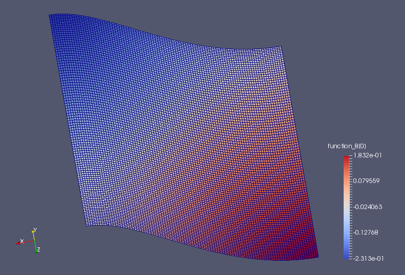
VTKFile("u.pvd").write(u)
An image of the solution is shown below.
A python script version of this demo can be found here.
References