Camassa-Holm equation

This tutorial was contributed by Colin Cotter.

The Camassa Holm equation [CH93] is an integrable 1+1 PDE which may be written in the form

\[m_t + mu_x + (mu)_x = 0, \quad u - \alpha^2u_{xx} = m,\]

solved in the interval \([a,b]\) either with periodic boundary conditions or with boundary conditions u(a)=u(b)=0; \(\alpha>0\) is a constant that sets a lengthscale for the solution. The solution is entirely composed of peaked solitons corresponding to Dirac delta functions in \(m\). Further, the solution has a conserved energy, given by

\[\int_a^b \frac{1}{2} u^2 + \frac{\alpha^2}{2} u_x^2\, \mathrm{d}x.\]

In this example we will concentrate on the periodic boundary conditions case.

A weak form of these equations is given by

\[ \begin{align}\begin{aligned}\int pm_t + pmu_x - p_xmu\, \mathrm{d}x=0, \quad \forall p,\\\int qu + \alpha^2q_xu_x - qm\, \mathrm{d}x=0, \quad \forall q.\end{aligned}\end{align} \]

Energy conservation then follows from substituting the second equation into the first, and then setting \(p=u\),

\[\begin{split}\dot{E} &= \frac{\mathrm{d}}{\mathrm{d}t}\int_a^b \frac{1}{2}u^2 + \frac{\alpha^2}{2}u_x^2\, \mathrm{d}x \\ &= \int_a^b uu_t + \alpha^2 u_xu_{xt}\, \mathrm{d}x, \\ &= \int_a^b um_t\, \mathrm{d}x, \\ &= \int_a^b -umu_x + u_xmu\, \mathrm{d}x = 0.\end{split}\]

If we choose the same continuous finite element spaces for \(m\) and \(u\) then this proof immediately extends to the spatial discretisation, as noted by [Mat10]. Further, it is a property of the implicit midpoint rule time discretisation that any quadratic conserved quantities of an ODE are also conserved by the time discretisation (see [Ise09], for example). Hence, the fully discrete scheme,

\[ \begin{align}\begin{aligned}\int p(m^{n+1}-m^n) + \Delta t(pm^{n+1/2}u^{n+1/2}_x - p_xm^{n+1/2}u^{n+1/2})\,\mathrm{d}x=0, \quad \forall p\in V,\\\int qu^{n+1/2} + \alpha^2q_xu^{n+1/2}_x - qm^{n+1/2}\, \mathrm{d}x=0, \quad \forall q \in V,\end{aligned}\end{align} \]

where \(u^{n+1/2}=(u^{n+1}+u^n)/2\), \(m^{n+1/2}=(m^{n+1}+m^n)/2\), conserves the energy exactly. This is a useful property since the energy is the square of the \(H^1\) norm, which guarantees regularity of the numerical solution.

As usual, to implement this problem, we start by importing the Firedrake namespace.

from firedrake import *

To visualise the output, we also need to import matplotlib.pyplot to display the visual output

try:
  import matplotlib.pyplot as plt
except:
  warning("Matplotlib not imported")

We then set the parameters for the scheme.

alpha = 1.0
alphasq = Constant(alpha**2)
dt = 0.1
Dt = Constant(dt)

These are set with type Constant so that the values can be changed without needing to regenerate code.

We use a periodic mesh of width 40 with 100 cells,

n = 100
mesh = PeriodicIntervalMesh(n, 40.0)

and build a mixed function space for the two variables.

V = FunctionSpace(mesh, "CG", 1)
W = MixedFunctionSpace((V, V))

We construct a Function to store the two variables at time level n, and subfunctions it so that we can interpolate the initial condition into the two components.

w0 = Function(W)
m0, u0 = w0.subfunctions

Then we interpolate the initial condition,

\[u^0 = 0.2\text{sech}(x-403/15) + 0.5\text{sech}(x-203/15),\]

into u,

x, = SpatialCoordinate(mesh)
u0.interpolate(0.2*2/(exp(x-403./15.) + exp(-x+403./15.))
               + 0.5*2/(exp(x-203./15.)+exp(-x+203./15.)))

before solving for the initial condition for m. This is done by setting up the linear problem and solving it (here we use a direct solver since the problem is one dimensional).

p = TestFunction(V)
m = TrialFunction(V)

am = p*m*dx
Lm = (p*u0 + alphasq*p.dx(0)*u0.dx(0))*dx

solve(am == Lm, m0, solver_parameters={
      'ksp_type': 'preonly',
      'pc_type': 'lu'
      }
   )

Next we build the weak form of the timestepping algorithm. This is expressed as a mixed nonlinear problem, which must be written as a bilinear form that is a function of the output Function w1.

p, q = TestFunctions(W)

w1 = Function(W)
w1.assign(w0)
m1, u1 = split(w1)
m0, u0 = split(w0)

Note the use of split(w1) here, which splits up a Function so that it may be inserted into a UFL expression.

mh = 0.5*(m1 + m0)
uh = 0.5*(u1 + u0)

L = (
(q*u1 + alphasq*q.dx(0)*u1.dx(0) - q*m1)*dx +
(p*(m1-m0) + Dt*(p*uh.dx(0)*mh -p.dx(0)*uh*mh))*dx
)

Since we are in one dimension, we use a direct solver for the linear system within the Newton algorithm. To do this, we assemble a monolithic rather than blocked system.

uprob = NonlinearVariationalProblem(L, w1)
usolver = NonlinearVariationalSolver(uprob, solver_parameters=
   {'mat_type': 'aij',
    'ksp_type': 'preonly',
    'pc_type': 'lu'})

Next we use the other form of subfunctions, w0.subfunctions, which is the way to split up a Function in order to access its data e.g. for output.

m0, u0 = w0.subfunctions
m1, u1 = w1.subfunctions

We choose a final time, and initialise a VTKFile object for storing u. as well as an array for storing the function to be visualised:

T = 100.0
ufile = VTKFile('u.pvd')
t = 0.0
ufile.write(u1, time=t)
all_us = []

We also initialise a dump counter so we only dump every 10 timesteps.

ndump = 10
dumpn = 0

Now we enter the timeloop.

while (t < T - 0.5*dt):
   t += dt

The energy can be computed and checked.

#
   E = assemble((u0*u0 + alphasq*u0.dx(0)*u0.dx(0))*dx)
   print("t = ", t, "E = ", E)

To implement the timestepping algorithm, we just call the solver, and assign w1 to w0.

#
   usolver.solve()
   w0.assign(w1)

Finally, we check if it is time to dump the data. The function will be appended to the array of functions to be plotted later:

#
   dumpn += 1
   if dumpn == ndump:
      dumpn -= ndump
      ufile.write(u1, time=t)
      all_us.append(Function(u1))

This solution leads to emergent peakons (peaked solitons); the left peakon is travelling faster than the right peakon, so they collide and momentum is transferred to the right peakon.

At last, we call the function plot on the final value to visualize it:

try:
  from firedrake.pyplot import plot
  fig, axes = plt.subplots()
  plot(all_us[-1], axes=axes)
except Exception as e:
  warning("Cannot plot figure. Error msg: '%s'" % e)

And finally show the figure:

try:
  plt.show()
except Exception as e:
  warning("Cannot show figure. Error msg: '%s'" % e)

Images of the solution at shown below.

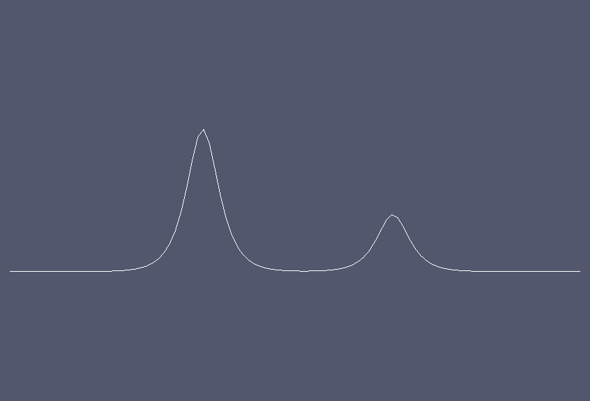
Solution at \(t = 0.\)

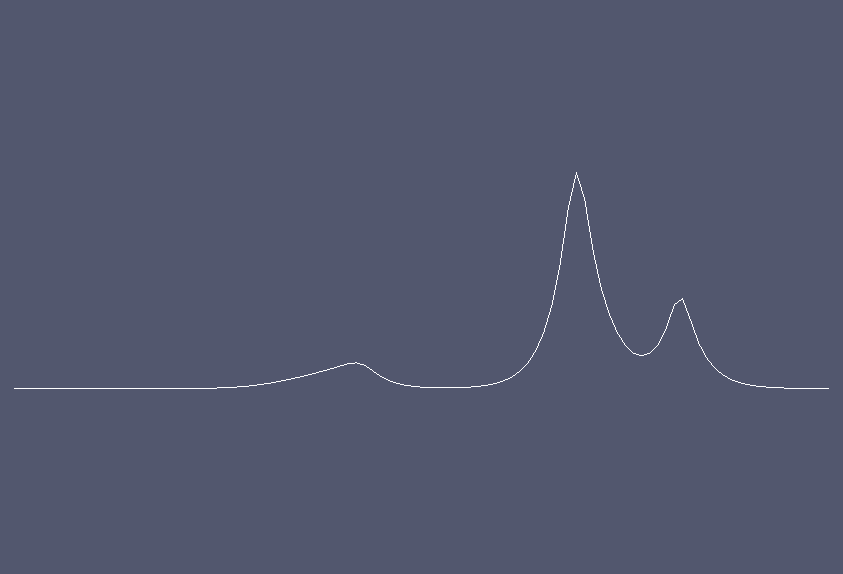
Solution at \(t = 2.5.\)

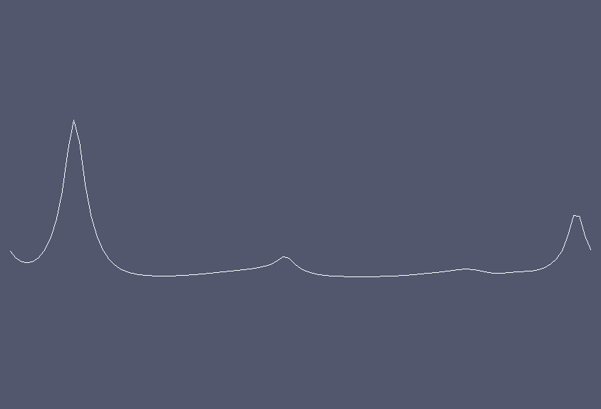
Solution at \(t = 5.3.\)

A python script version of this demo can be found here.

References

[CH93]

Roberto Camassa and Darryl D. Holm. An integrable shallow water equation with peaked solitons. Physical Review Letters, 71(11):1661, 1993.

[Ise09]

Arieh Iserles. A first course in the numerical analysis of differential equations. Number 44 in Cambridge Texts in Applied Mathematics. Cambridge University Press, 2009.

[Mat10]

Takayasu Matuso. A Hamiltonian-conserving Galerkin scheme for the Camassa-Holm equation. Journal of Computational and Applied Mathematics, 234(4):1258–1266, 2010.